5  Accounting for Zero Inflation

Another extension, called hhh4ZI, of hhh4 models is to include a zero-inflation component, which accounts for excess zeros in infectious disease surveillance data.

5.1 Mathematical Formulation

The standard hhh4 model usually assumes that the disease counts follow a negative binomial distribution with conditional mean \(\mu_{it}\). In order to account for a greater number of zeros than expected under this model, Lu and Meyer (2023) proposed a zero-inflation extension that combines the endemic-epidemic model with a point mass at zero.

The number of observed cases \(Y_{it}\) is assumed to follow a zero-inflated negative binomial distribution, combining:

• standard endemic-epidemic negative binomial model with probability mass function \(f(y_{it}; \mu_{it}, \psi)\)
• a logit model with zero-inflation probability \(\gamma_{it}\).

The distribution of \(Y_{it}\) is given by

\[ P(Y_{it} = y) = \begin{cases} \gamma_{it} + (1 - \gamma_{it}) f(0; \mu_{it}, \psi), & \text{if } y = 0, \\ (1 - \gamma_{it}) f(y; \mu_{it}, \psi), & \text{if } y > 0. \end{cases} \]

The parameter \(\gamma_{it}\) describes the probability that a zero count is a structural zero. When \(\gamma_{it}=0\), the model reduces to the standard hhh4 formulation.

The zero-inflation probability is modelled using a logit link, \[ \operatorname{logit}(\gamma_{it}) = \beta_0^{(\gamma)} + b_i^{(\gamma)} + z_{it}^{(\gamma)}\beta^{(\gamma)}, \]

and may include covariates \(z_{it}\). For example, an autoregressive term based on previous case counts can be used to reflect how recent local infections affect the probability of excess zeros. For further details, see Lu and Meyer (2023).

5.2 Using Surveillance

To fit a zero-inflated model in hhh4ZI, we need to add the zero-inflation component zi to our control list. In this example we use the default formulation for zi, which includes autoregression as a covariate (lag = 1).

noroEEziModel <- c(noroEEModel, zi = list(f = ~ 1, lag = 1))
noroEEziModel$end <- list(f = addSeason2formula(f = ~ 1), offset = population(noroBE))
noroEEziModel$ne <- list(f = ~ 1, weights = neighbourhood(noroBE) >= 1)

To fit the model we use the function hhh4ZI() and look at the summary:

noroEEziFit <- hhh4ZI(noroBE, noroEEziModel)
summary(noroEEziFit)

Call: 
hhh4ZI(stsObj = noroBE, control = noroEEziModel)

Coefficients:
                        Estimate   Std. Error
ar.1                    -0.847269   0.048217 
ne.1                    -4.392670   0.246073 
end.1                    3.096850   0.080279 
end.sin(2 * pi * t/52)  -0.008734   0.048608 
end.cos(2 * pi * t/52)  -0.923716   0.045399 
zi.1                    -5.725895   5.736761 
zi.AR(1)                -0.247597   0.422392 
overdisp                 0.224832   0.014706 

Log-likelihood:   -5853.75 
AIC:              11723.5 
BIC:              11770.04 

Number of units:        12 
Number of time points:  207 

We can directly see, that the standard error for both zero-inflation parameters is bigger than the estimate itself, making it not significant for our model.

In hhh4ZI we can plot a map of the zero-inflation probability:

plot(noroEEziFit, type = "maps", which = "zi")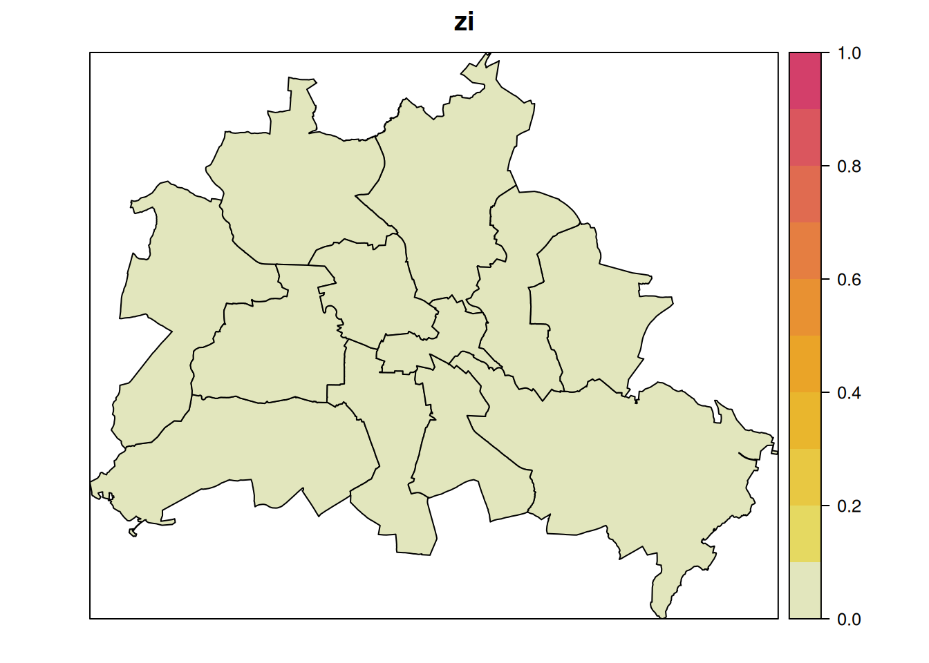

From the map, we see that the estimated zero-inflation probabilities are very low across all districts. This indicates that the additional zero-inflation component contributes little to the fitted model and suggests that the underlying negative binomial distribution already captures the observed frequency of zeros reasonably well.

5.3 Using RTMB

To add a zero inflation component to the objective function, we use an additional package called RTMBdist. Here, a zero-inflated negative binomial distribution is already implemented and we can use the function dzinbinom() directly.

For the zero-inflation probability, we add the parameter \(\gamma\) which we call zi.1. We also include an autoregressive term in the zero-inflation component as in the default hhh4ZI model (zi.AR1).

library(RTMBdist)

meanEEzi <- function(parms, data){
  ## ENDEMIC
  s_vec <- parms$end.sin * data$Ssin + parms$end.cos * data$Scos
  end.exppred <- exp(parms$end.1 + s_vec + log(data$pop))
  end <- end.exppred[-1, ]

  ## EPIDEMIC
  Y_lag <-  data$Y[1:(data$n_time - 1), ]
  ## AR
  ar.exppred <- exp(parms$ar.1) 
  ar <- ar.exppred * Y_lag
  ## NE
  ## same weights for all neighbours
  W <- data$W_n >= 1
  ne.exppred <- exp(parms$ne.1) 
  ne <- ne.exppred * (Y_lag %*% W)

  ## ZI
  zi.pre <- parms$zi.1 + parms$zi.AR1 * Y_lag # autoreg in ZI
  REPORT(zi.pre)

  return(list(mu = end + ar + ne,
              end = end,
              epi = ar + ne,
              epi.ar = ar, epi.ne = ne,
              end.exppred = end.exppred,
              ar.exppred = ar.exppred,
              ne.exppred = ne.exppred,
              zi = zi.pre,
              neW = W))
}

objectiveEEzi <- function(parms, data) {

  Y <- OBS(data$Y)

  ## helper function for mean calculation
  fit <- meanEEzi(parms, data)
  
  ## negative log likelihood
  nll <- - sum(dzinbinom2(Y[-1, ], mu = fit$mu, size = exp(parms$log_overdispersion), zeroprob = plogis(fit$zi), log = TRUE))
  nll
}

Both zero-inflation parameters need to be added to the parms list.

parms <-list(
  ar.1  = 0, 
  ne.1 = 0,
  end.1 = 0,
  end.sin = 0, 
  end.cos = 0,
  zi.1 = 0,
  zi.AR1 = 0, 
  log_overdispersion = 0
)

We again process the objective function, fit the model and calculate uncertainties.

objEEzi <- MakeADFun(cmb(objectiveEEzi, data), parms)

ptm <- proc.time() # track runtime
## fit the model 
optEEzi <- nlminb( objEEzi$par, objEEzi$fn, objEEzi$gr)
## calculate uncertainties
sdrEEzi <- sdreport(objEEzi)
runtime_EEzi <- proc.time() - ptm

We use summary() to get the estimates of the RTMB model.

summary(sdrEEzi)

                       Estimate Std. Error
ar.1               -0.847268975 0.04821741
ne.1               -4.392669554 0.24607169
end.1               3.096849653 0.08027834
end.sin            -0.008733584 0.04860774
end.cos            -0.923715153 0.04539901
zi.1               -5.725799925 5.73619451
zi.AR1             -0.247604388 0.42238211
log_overdispersion  1.492404306 0.06540972

We can get the zero-inflation probability (without SEs) like this:

(ZIdistricts <- colMeans(plogis(objEEzi$report()$zi.pre)))

        chwi         frkr         lich         mahe         mitt         neuk 
0.0014411274 0.0019246193 0.0015566941 0.0016415926 0.0015583534 0.0015719921 
        pank         rein         span         zehl         scho         trko 
0.0010116510 0.0014728229 0.0017253190 0.0009966004 0.0011953585 0.0014600631 

We can plot the zero-inflation probability as a map using sf. In the sts object noroBE the map data is of class SpatialPolygonsDataFrame from the sp package. Since this package is not actively developed anymore, and users are engouraged to use the modern sf package, we use the now standard sf package for geo data. See this article for more information. Using ggplot2’s geom_sf() function we can plot the zero-inflation probability easily. We just need to make sure the order is the same.

library(sf)

Linking to GEOS 3.12.1, GDAL 3.8.4, PROJ 9.4.0; sf_use_s2() is TRUE

class(noroBE@map)

[1] "SpatialPolygonsDataFrame"
attr(,"package")
[1] "sp"

mapBE <- st_as_sf(noroBE@map)
all.equal(rownames(mapBE), names(ZIdistricts))

[1] TRUE

mapBE$ZI <- ZIdistricts

ggplot(mapBE) +
  geom_sf(aes(fill = ZI))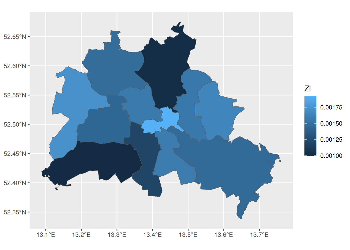

To make it look like the surveillance::plot(), we can adjust it:

ggplot(mapBE) +
  geom_sf(aes(fill = ZI)) +
  scale_fill_stepsn(
    colors = surveillance:::.hcl.colors(10),
    breaks = seq(0, 1, 0.1),
    limits = c(0, 1),
    guide = guide_colorbar(barheight = unit(1, "npc"))
  ) +
  labs(title = "zi", fill = NULL) +
  theme_bw() +
  theme(
    axis.text = element_blank(),
    axis.ticks = element_blank(),
    title = element_text(size = 14, face = "bold"),
    legend.text = element_text(size = 14)
  )

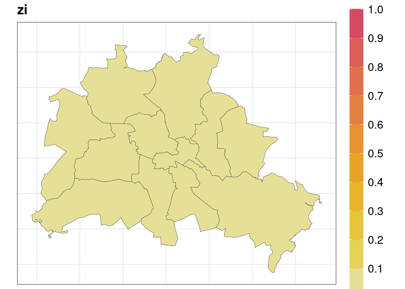
The mean of the zero-inflation probability for each district is below 1%, as we already saw in the map of the hhh4ZI model.

5.4 Comparison Table

Parameter estimates and runtime for <code>hhh4</code> and <code>RTMB</code> implementations with standard errors (SE) in brackets and differences between both implementations.

	hhh4	RTMB	diff.
Parameters
ar.1	-0.847269163 (0.048217442)	-0.847268975 (0.048217409)	-1.88e-07 (3.29e-08)
ne.1	-4.392670022 (0.246072738)	-4.392669554 (0.246071686)	-4.68e-07 (1.05e-06)
end.1	3.096849658 (0.080278576)	3.096849653 (0.080278342)	5.37e-09 (2.34e-07)
end.sin(2 * pi * t/52)	-0.008733742 (0.048607787)	-0.008733584 (0.04860774)	-1.58e-07 (4.77e-08)
end.cos(2 * pi * t/52)	-0.923715523 (0.045399051)	-0.923715153 (0.045399011)	-3.7e-07 (4e-08)
zi.1	-5.725895325 (5.736760685)	-5.725799925 (5.736194508)	-9.54e-05 (0.000566)
zi.AR(1)	-0.247596514 (0.422391819)	-0.247604388 (0.422382113)	7.87e-06 (9.71e-06)
-log(overdisp)	1.492402992 (0.065409839)	1.492404306 (0.065409723)	-1.31e-06 (1.16e-07)
Metrics
Log-Likelihood	-5853.748267687	-5853.748267688	0
Runtime (seconds)	0.319	0.111	0.208

Here both parameter estimates are quite similar, as well as the time it takes.

Lu, Junyi, and Sebastian Meyer. 2023. “A Zero-Inflated Endemic–Epidemic Model with an Application to Measles Time Series in Germany.” Biometrical Journal 65 (8): 2100408. https://doi.org/10.1002/bimj.202100408.