noroEEModel <-   list(
    end = list(f = addSeason2formula(f = ~ -1 + fe(1, unitSpecific = TRUE))),
    ar = list(f = ~ 1),
    ne = list(
        f = ~ 1,
        weights = W_powerlaw(maxlag = max(neighbourhood(noroBE)),
                             initial = c("logd" = log(2)),
                             normalize = TRUE, log = TRUE)),
    family = "NegBin1",
    data = list(t = 1:nrow(noroBE) - 1)
)2 Full Endemic-Epidemic Models with Seasonality and Spatial Power Law
Now that we have a valid endemic-only model in RTMB, we expand this basic model to the full endemic-epidemic model structure. We build a model with autoregression and seasonal variation.
2.1 Mathematical Formulation
In the standard hhh4 endemic-epidemic model formulation, the conditional mean \(\mu_{it}\) for the counts \(Y_{it}\) is decomposed into two components: an endemic component (\(\nu_{it}\)), that is the background level, and an epidemic component, that is observation-driven and further splitted into an autoregressive component (\(\lambda_{it}\)) and a spatiotemporal component (\(\phi_{it}\)):
\[ \mu_{it} = \nu_{it} + \lambda_{it} Y_{i,t-1} + \phi_{it} \sum_{j \neq i} w_{ji} Y_{j,t-1} \]
Where \(w_{ji}\) are the spatial weights for the neighborhood.
2.1.1 Adding Seasonality via Harmonic Terms
Seasonality is typically modeled by incorporating sinusoidal waves into the log-linear predictor of the components. For a seasonal period \(S\) (where \(S = 52\) for weekly data), a first-order harmonic wave is written as:
\[\log(\nu_{it}) = \beta_0 + b_i + \gamma \sin\left(\frac{2\pi}{S} t\right) + \delta \cos\left(\frac{2\pi}{S} t\right)\]
2.1.2 Modeling Spatial Spread via a Power Law
For the spatial spread, we model the neighborhood weights \(w_{ji}\) using a spatial power law. Following the implementation from Meyer and Held (2014), we use the neighborhood order \(o_{ji}\) as a discrete distance measure. The weights are modeled with a decay parameter \(d > 0\):
\[w_{ji} = o_{ji}^{-d} \quad \text{for } j \neq i\]
The raw weights are row-normalized so that the total spatial contribution from any source district \(j\) sums to 1:
\[w_{ji} = \frac{o_{ji}^{-d}}{\sum_{k=1}^{I} o_{jk}^{-d}}\]
where \(o_{jk}^{-d} = 0\) if \(j=k\).
Higher \(d\): transmission mainly local (as \(d \to \infty\), it simplifies to first-order adjacency)
Lower \(d\): longer-range transmission across the neighborhood
2.2 Using surveillance
In hhh4, adding autoregressive and spatiotemporal components, seasonality and power-law weights is straightforward. The surveillance package provides the helper function addSeason2formula() to generate the harmonic terms for the endemic component, and W_powerlaw() to handle the neighborhood order decay. We get the neighborhood order matrix from our sts object as our distance metric \(o_{ji}\) using neighbourhood(). First, we create a new control object. To add seasonal terms, we need to add t, the total number of weeks to the data list. This time we add region-specific fixed effects to account for heterogenity between the different Berlin districts in the endemic component.
We fit the model using hhh4() and can look at the summary:
noroEEFit <- hhh4(noroBE, noroEEModel)
summary(noroEEFit)
Call:
hhh4(stsObj = noroBE, control = noroEEModel)

Coefficients:
                        Estimate  Std. Error
ar.1                    -1.16764   0.06826
ne.1                    -1.55390   0.15658
end.sin(2 * pi * t/52)  -0.06542   0.04200
end.cos(2 * pi * t/52)  -0.99974   0.04025
end.1.chwi               0.51900   0.12837
end.1.frkr              -0.37488   0.27108
end.1.lich               0.53092   0.12293
end.1.mahe               0.38298   0.15202
end.1.mitt               0.45502   0.13504
end.1.neuk               0.40716   0.13710
end.1.pank               1.27522   0.08416
end.1.rein               0.62801   0.11862
end.1.span               0.15550   0.17280
end.1.zehl               1.42264   0.08182
end.1.scho               0.95372   0.09946
end.1.trko               0.64516   0.11861
neweights.logd          -1.06967   1.44845
overdisp                 0.19092   0.01211

Log-likelihood:   -5772.66
AIC:              11581.31
BIC:              11686.03

Number of units:        12
Number of time points:  207
Notably, the spatial decay parameter neweights.logd is statistically non-significant due to a large standard error, indicating that the decay rate cannot be reliably estimated from the data. On the original scale, the estimate exponentiates to \(d =\) 0.3431219. This implies almost uniform transmission weights across neighbouring districts. Although this parameter has limited statistical identifiability here, we will keep it in the current model to demonstrate the implementation of the power-law formulation.
2.3 Using RTMB
Since we want the RTMB objective function to be the pure likelihood evaluation, we add additional information for the seasonal terms and the neighbourhood to the data list.
## add predefined seasonal terms
data$Ssin <- sin(2 * pi * (0:(n_time-1))/52) # seasonality outside of AD objective Fun
data$Scos <- cos(2 * pi * (0:(n_time-1))/52) # starts from 0

## add neighbourhood matrix
data$W_n <- neigh
In the objective function, we first transform the parameters and define the power-law function. We then loop over the time points to calculate the three model components and \(\mu_{it}\).
For the endemic component, we calculate the seasonality scalar s_t for each time point \(t\) and add it to the endemic fixed-effect vector \(b_i\).
For the epidemic components, we multiply the lagged counts vector \(Y_{i}\) at \(t-1\) by the normalized neighbourhood weight matrix from the power law W_norm, which needs to be transposed. This gives the weighted sum of neighbouring cases Y_neigh. The lagged counts Y_lag are multiplied by the autoregressive intercept ar.1 (corresponding to \(\beta_0\) in the formula) and Y_neigh by the spatiotemporal intercept ne.1. Summing these three components gives the vector \(\mu_{i}\) at time \(t\).
\(\mu_{i}\) is then used to calculate the negative binomial density of \(Y_{i}\). The resulting log-densities are summed over \(i\) and then over all time points to obtain the negative log-likelihood.
objectiveEE <- function(parms, data) {

  getAll(parms, data) # makes data list and parameters visible inside the function

  ## tells RTMB that that Y is the response
  Y <- OBS(Y)

  ## Initialize negative log likelihood
  nll <- 0

  ## transform parameters
  exp_ar.1 <- exp(ar.1)
  exp_ne.1 <- exp(ne.1)
  neweights.d <- exp(neweights.logd)
  exp_overdispersion <- exp(log_overdispersion)

  ## power-law
  W <- W_n^(-neweights.d)
  diag(W) <- 0 # enforce w_jj = 0 since it is Inf otherwise
  W_norm <- W / rowSums(W) # normalize rows

  for (t in 2:n_time) {
    ## ENDEMIC
    ## sesonality
    s_t <- end.sin * Ssin[t] + end.cos * Scos[t]
    ## endemic log linear predictor
    nu_t <- end.fe + s_t
    ## EPIDEMIC
    Y_lag <- Y[t-1, ]
    Y_neigh <- as.vector(t(W_norm) %*% Y_lag)
    ## MU
    mu_t <- exp(nu_t) + exp_ar.1 * Y_lag + exp_ne.1 * Y_neigh
    ## negative log likelihood
    nll <- nll - sum(dnbinom2(Y[t, ], mu = mu_t, size = exp_overdispersion, log = TRUE))
  }
  return(nll)
}
parms <- list(
ar.1 = 0,
ne.1 = 0,
end.sin = 0,
end.cos = 0,
end.fe = rep(0, data$n_unit),
neweights.logd = log(2),
log_overdispersion = 0
)Then, we process the objective function, fit the model and calculate uncertainties as before.
## process objective function
objEE <- MakeADFun(cmb(objectiveEE, data), parms)

## fit the model
ptm <- proc.time() # track runtime for optimization and uncertainties
optEE <- nlminb( objEE$par, objEE$fn, objEE$gr)

## calculate uncertainties
sdrEE <- sdreport(objEE)
runtime_EE <- proc.time() - ptm
The estimates from our RTMB model:
summary(sdrEE) Estimate Std. Error
ar.1 -1.16764299 0.06826149
ne.1 -1.55390611 0.15658238
end.sin -0.06541688 0.04199941
end.cos -0.99973857 0.04025159
end.fe 0.51900651 0.12836868
end.fe -0.37484675 0.27107951
end.fe 0.53092116 0.12293123
end.fe 0.38295737 0.15202868
end.fe 0.45503922 0.13504054
end.fe 0.40716897 0.13710142
end.fe 1.27522363 0.08416465
end.fe 0.62803053 0.11861570
end.fe 0.15548316 0.17280528
end.fe 1.42262843 0.08182223
end.fe 0.95371805 0.09945605
end.fe 0.64514915 0.11861535
neweights.logd -1.07005799 1.44920436
log_overdispersion 1.65590898 0.06342688We will compare the estimates in a table at the end of this chapter. In the next chapter (Chapter 3), we can see a solution, where each parameter has an individual name.
2.3.1 Checking Correctness of the Implementation using Simulation
As suggested in the vignette of RTMB we could check the it’s correctness using checkConsitency, where 100 datasets are simulated and gradients for each replicate are calculated. For further details see vignette("RTMB-introduction"). But as explained later on in detail (Section 2.5), the RTMB simulation function is not working with autoregressive models.
# set.seed(1)
# chk <- checkConsistency(objEE)
# chk
2.3.2 Get Fitted Values
In RTMB we could use the ADREPORT() function to directly get the estimates for \(\mu\) (intermediate calculation) along with their uncertainties. But, this slows down the model fitting quite a bit.
If we add ADREPORT(mu) and initialize a matrix mu where we save all \(\mu_{it}\) for each time point, our objective function looks like this:
objectiveEEmu <- function(parms, data) {

  getAll(parms, data) # makes data list and parameters visible inside the function

  ## tells RTMB that that Y is the response
  Y <- OBS(Y)

  ## initialize mu matrix
  mu <- matrix(NA, n_time, n_unit)

  ## Initialize negative log likelihood
  nll <- 0

  ## transform parameters
  exp_ar.1 <- exp(ar.1)
  exp_ne.1 <- exp(ne.1)
  neweights.d <- exp(neweights.logd)
  exp_overdispersion <- exp(log_overdispersion)

  ## power-law
  W <- W_n^(-neweights.d)
  diag(W) <- 0 # enforce w_jj = 0 since it is Inf otherwise
  W_norm <- W / rowSums(W) # normalize rows

  for (t in 2:n_time) {
    ## ENDEMIC
    ## sesonality
    s_t <- end.sin * Ssin[t] + end.cos * Scos[t]
    ## endemic log linear predictor
    nu_t <- end.fe + s_t
    ## EPIDEMIC
    Y_lag <- Y[t-1, ]
    Y_neigh <- as.vector(t(W_norm) %*% Y_lag)
    ## MU
    mu_t <- exp(nu_t) + exp_ar.1 * Y_lag + exp_ne.1 * Y_neigh

    ## negative log likelihood
    nll <- nll - sum(dnbinom2(Y[t, ], mu = mu_t, size = exp_overdispersion, log = TRUE))

    mu[t, ] <- mu_t # fill mu matrix

  }
  ADREPORT(mu)
  return(nll)
}
The fitting and uncertainty calculation takes 0.996 seconds longer.
When using ADREPORT(), we can get the estimated values for \(\mu_{it}\) after we run sdreport():
str(as.list(sdrEEmu, "Est", report=TRUE)) # ADREPORT estimatesList of 1
$ mu: num [1:208, 1:12] NA 1.62 2.16 2.61 1.02 ...
- attr(*, "what")= chr "Estimate"str(as.list(sdrEEmu, "Std", report=TRUE)) # ADREPORT uncertaintiesList of 1
$ mu: num [1:208, 1:12] 0 0.077 0.0981 0.1159 0.0863 ...
- attr(*, "what")= chr "Std. Error"Why does ADREPORT() slow it down? When we include ADREPORT(), RTMB tracks the values of \(\mu_{it}\) and the standard errors are calculated using the Delta Method.
2.3.2.1 Alternatives to ADREPORT()
- Using
REPORT()
If we want to get the fitted values without uncertainties we can just use REPORT():
objectiveEEre <- function(parms, data) {

  getAll(parms, data) # makes data list and parameters visible inside the function

  ## tells RTMB that that Y is the response
  Y <- OBS(Y)

  ## initialize mu matrix
  mu <- matrix(NA, n_time, n_unit)

  ## Initialize negative log likelihood
  nll <- 0

  ## transform parameters
  exp_ar.1 <- exp(ar.1)
  exp_ne.1 <- exp(ne.1)
  neweights.d <- exp(neweights.logd)
  exp_overdispersion <- exp(log_overdispersion)

  ## power-law
  W <- W_n^(-neweights.d)
  diag(W) <- 0 # enforce w_jj = 0 since it is Inf otherwise
  W_norm <- W / rowSums(W) # normalize rows

  for (t in 2:n_time) {
    ## ENDEMIC
    ## sesonality
    s_t <- end.sin * Ssin[t] + end.cos * Scos[t]
    ## endemic log linear predictor
    nu_t <- end.fe + s_t
    ## EPIDEMIC
    Y_lag <- Y[t-1, ]
    Y_neigh <- as.vector(t(W_norm) %*% Y_lag)
    ## MU
    mu_t <- exp(nu_t) + exp_ar.1 * Y_lag + exp_ne.1 * Y_neigh

    ## negative log likelihood
    nll <- nll - sum(dnbinom2(Y[t, ], mu = mu_t, size = exp_overdispersion, log = TRUE))

    mu[t, ] <- mu_t # fill mu matrix

  }
  REPORT(mu)
  return(nll)
}
The time it takes for model fitting and reporting is not different from before, when we did not use any report function (-0.005 seconds)
We will get the estimated values of \(\mu_{it}\) via calling:
head(objEEre$report()$mu) [,1] [,2] [,3] [,4] [,5] [,6] [,7] [,8]
[1,] NA NA NA NA NA NA NA NA
[2,] 1.616668 0.9630774 1.280396 0.8620690 2.161518 0.9379537 2.283679 1.372407
[3,] 2.163218 1.4987135 1.794636 1.0729153 1.811772 2.3417269 2.798814 1.310088
[4,] 2.614722 1.6280058 1.400714 0.9756067 1.119241 1.0599658 2.133702 1.507492
[5,] 1.023032 0.6068389 1.255471 0.8399196 1.825177 0.9048245 2.310658 1.062968
[6,] 1.952061 2.1370278 1.087532 0.9415431 1.939391 1.0128952 2.184750 1.452053
[,9] [,10] [,11] [,12]
[1,] NA NA NA NA
[2,] 0.8057862 2.780602 2.826277 1.343797
[3,] 1.3501069 5.073434 2.826166 1.586639
[4,] 2.0974451 3.260450 2.388315 2.041299
[5,] 0.7901634 4.002369 2.259040 1.040185
[6,] 1.1177584 2.109731 2.071921 2.029116- Using a helper function.
We could also create an external helper function assurveillancedoes withmeanHHH()and use this inside our objective and outside of it later to get the fitted mean and component decomposition without the standard error calculation and AD taping:
meanEE <- function(parms, data){
  ## ENDEMIC
  fe_mat <- matrix(parms$end.fe, nrow = data$n_time, ncol = data$n_unit, byrow = TRUE)
  s_vec <- parms$end.sin * data$Ssin + parms$end.cos * data$Scos
  end.exppred <- exp(fe_mat + s_vec)
  end <- end.exppred[- 1, ]

  ## EPIDEMIC
  Y_lag <-  data$Y[1:(data$n_time - 1), ]
  ar.exppred <- exp(parms$ar.1)
  ar <- ar.exppred * Y_lag

  W <- data$W_n^(-exp(parms$neweights.logd))
  diag(W) <- 0
  W_norm <- W / rowSums(W)
  ne.exppred <- exp(parms$ne.1)
  ne <- ne.exppred * (Y_lag %*% W_norm)

  return(list(mu = end + ar + ne,
              end = end,
              epi = ar + ne,
              epi.ar = ar, epi.ne = ne,
              end.exppred = end.exppred,
              ar.exppred = ar.exppred,
              ne.exppred = ne.exppred,
              neW = W_norm))
}
Note following differences:
Vectorization: Unlike the loop in
objectiveEEmu(), this function evaluates all time points simultaneously via matrix operations.No
getAll(): We explicitly use parms$ and data$ syntax.
We can now rewrite our objective function using the helper:
objectiveEEh <- function(parms, data) {

  ## tells RTMB that that Y is the response
  data$Y <- OBS(data$Y)

  fit <- meanEE(parms, data)

  ## negative log likelihood
  nll <- - sum(dnbinom2(data$Y[-1, ], mu = fit$mu, size = exp(parms$log_overdispersion), log = TRUE))

  return(nll)
}
By switching to this vectorized, modularized objective function, the fitting process takes -0.065 seconds less than before.
To extract our fitted means (and decomposition), we pass the optimized parameter estimates directly to our helper function. Although we get a named vector as output in the sdreport object, it needs to be a list, as the RTMB objective works with a parameter list as input.
## get estimates for mu
est <- split(sdrEEh$par.fixed, names(sdrEEh$par.fixed)) # needs to be a named list but is a named vector...
ptm <- proc.time()
fitted.val <- meanEE(est, data)
runtime_mu <- proc.time() - ptm
This takes only 0.003 seconds. The differences between the estimates for \(\mu\) from the hhh4 model to the RTMB model are negligible, with a maximum absolute difference of 1.3e-04.
Note: We could have used REPORT() or ADREPORT()for every “intermediate calculation” we need, such as: REPORT(fit$mu), REPORT(fit$end), REPORT(fit$epi), too.
The reported estimated \(\mu\) and component decomposition can then be plotted similar as with plot.hhh4() using base R or ggplot2.
2.3.2.2 Plotting in Base R
To plot the (overall) fitted values as decomposed plot, we first build a matrix with the component proportions and use cumsum and polygons() to plot the components on top of each other (as done in plot.hhh4(type = "fitted", total = TRUE)).
## aggregated fitted and observed values

plot.RTMBfit <- function(fitted.val, data) {
  observed <- rowSums(data$Y[2:nrow(data$Y), ])
  fitted <- rowSums(fitted.val$mu)

  ### base R
  fitted.val_matrix <- cbind(
    endemic = rowSums(fitted.val$end),
    autoregression = rowSums(fitted.val$epi.ar),
    spatiotemporal = rowSums(fitted.val$epi.ne)
  )
  time   <- 1:nrow(fitted.val$epi.ar)

  ## cumulative sum across rows (as plot.hhh4())
  fitted.val_cum <- t(apply(fitted.val_matrix, 1, cumsum))

  ## hhh4 colors
  comp_col <-  c(
    endemic = "grey85",
    autoregression = "blue",
    spatiotemporal = "orange"
  )

  ## plot window
  plot(range(time), c(0, max(observed)),
       type = "n", # blank plot
       xlab = "",
       ylab = "No. infected",
       main = "Overall")

  ## draw polygons
  ## spatiotemporal is drawn first
  for (comp in ncol(fitted.val_cum):1) {
    polygon(
      x = c(time[1], time, time[length(time)]),
      y = c(0, fitted.val_cum[, comp], 0),
      col = comp_col[comp],
      border = NA
    )
  }

  ## observed values as points
  points(x = time, y = observed, col = "black", pch = 16, cex = 0.7)

  ## add legend
  legend("topright", legend = colnames(fitted.val_matrix), col = comp_col, lty = 1, lwd = 6 ,bty = "n")
}
plot.RTMBfit(fitted.val, data)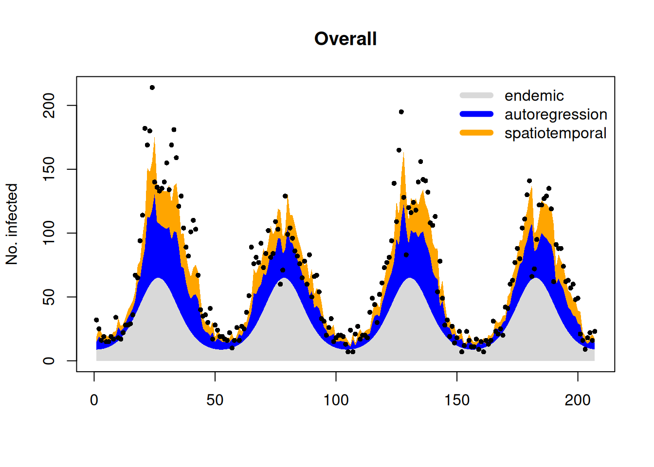
This gives a similar plot as plot.hhh4() for hhh4 objects:
plot(noroEEFit, type = "fitted", total = TRUE)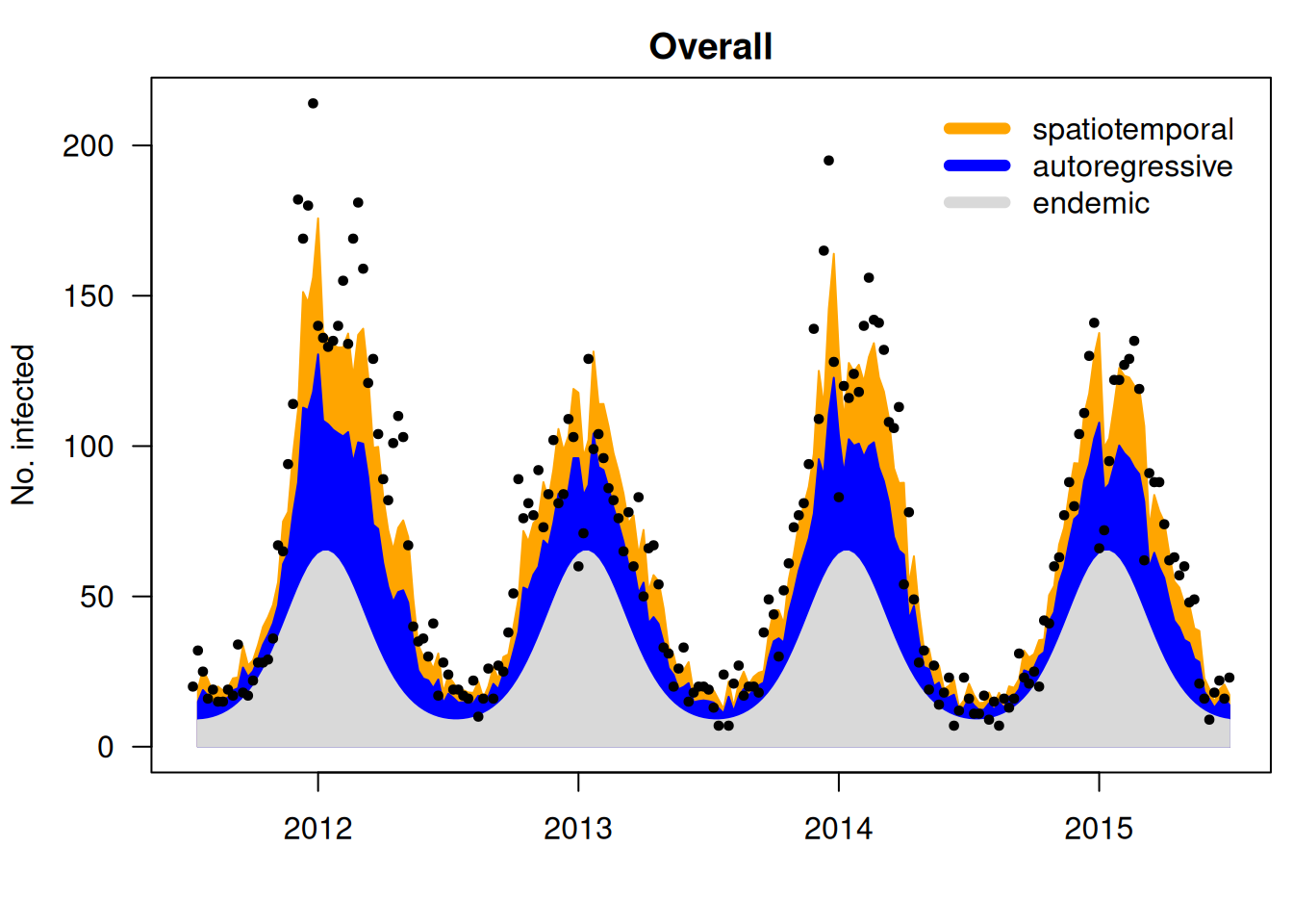
2.3.2.3 Ploting with ggplot2
We can also use ggplot2 to get a similar plot. But we need to transform the decompostion data into a long data.frame format.
# data.frame containing aggregated (district) component proportions
decomposition <- data.frame(
  time = 1:nrow(fitted.val$mu),
  observed = rowSums(data$Y[2:nrow(data$Y), ]),
  fitted = rowSums(fitted.val$mu),
  endemic = rowSums(fitted.val$end),
  autoregressive = rowSums(fitted.val$epi.ar),
  spatiotemporal = rowSums(fitted.val$epi.ne)
)

comp_col <-  c(
  endemic = "grey85",
  autoregression = "blue",
  spatiotemporal = "orange"
)

## shape it into long data.frame to plot proportions with ggplot()
fitted.val_long <- reshape(
    decomposition,
    direction = "long",
    idvar = "time",
    varying = list(names(decomposition)[4:6]),
    v.names = "Value",
    timevar = "Component",
    times = names(comp_col)
)
fitted.val_long$Component <- factor(fitted.val_long$Component,levels = names(comp_col))

### ggplot2
ggplot(fitted.val_long, aes(y = Value, x = time, fill = Component)) +
  geom_area(position = position_stack(reverse = TRUE)) +
  scale_fill_manual(values = comp_col) + # same colors as hhh4()
  geom_point(aes(y = observed), show.legend = FALSE) +
  theme_bw() +
  labs(x = "", y = "No. infected") +
  theme(legend.position = c(0.89, 0.89),
        legend.background = element_blank(),
        legend.title = element_blank())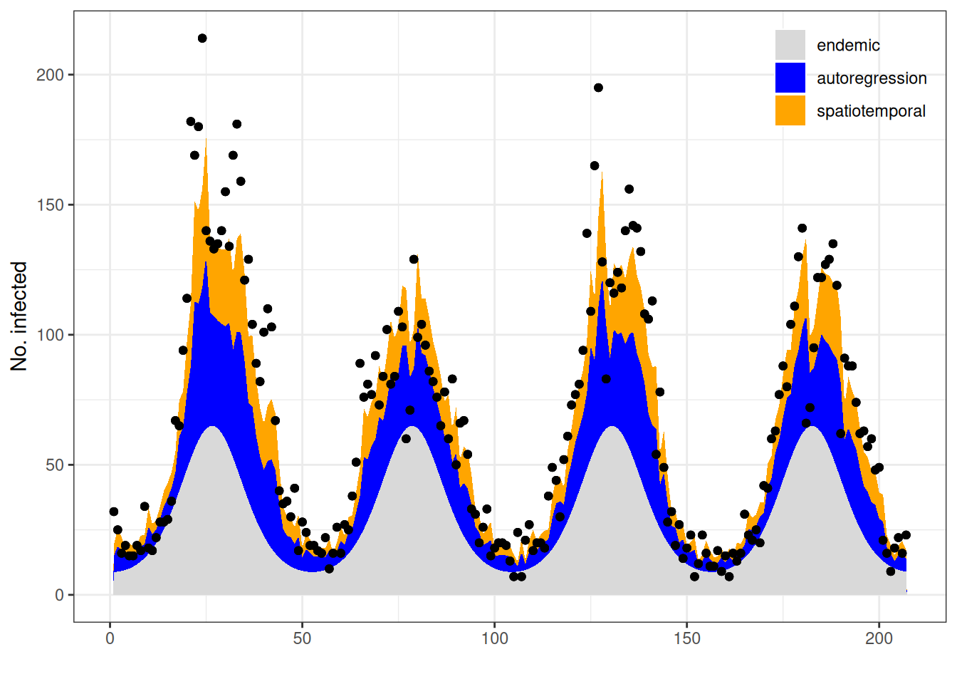
2.4 Comparison Table
To compare the hhh4 and RTMB models we use this table:
| hhh4 | RTMB | diff. | |
|---|---|---|---|
| Parameters | |||
| ar.1 | -1.167644189 (0.068261432) | -1.167642988 (0.068261492) | -1.2e-06 (-5.95e-08) |
| ne.1 | -1.553904841 (0.15658155) | -1.553906114 (0.156582379) | 1.27e-06 (-8.29e-07) |
| end.sin(2 * pi * t/52) | -0.065417196 (0.041999309) | -0.065416881 (0.041999406) | -3.15e-07 (-9.63e-08) |
| end.cos(2 * pi * t/52) | -0.999739884 (0.040251534) | -0.999738569 (0.040251593) | -1.31e-06 (-5.94e-08) |
| end.1.chwi | 0.51900144 (0.12836812) | 0.519006514 (0.128368682) | -5.07e-06 (-5.62e-07) |
| end.1.frkr | -0.374880949 (0.271078127) | -0.374846748 (0.271079515) | -3.42e-05 (-1.39e-06) |
| end.1.lich | 0.530921738 (0.122930881) | 0.530921158 (0.122931226) | 5.8e-07 (-3.44e-07) |
| end.1.mahe | 0.382981505 (0.152016225) | 0.382957366 (0.15202868) | 2.41e-05 (-1.25e-05) |
| end.1.mitt | 0.455023423 (0.135040563) | 0.455039223 (0.135040539) | -1.58e-05 (2.38e-08) |
| end.1.neuk | 0.407164447 (0.13710241) | 0.407168969 (0.137101416) | -4.52e-06 (9.94e-07) |
| end.1.pank | 1.275223348 (0.084164627) | 1.275223628 (0.084164645) | -2.8e-07 (-1.82e-08) |
| end.1.rein | 0.62801064 (0.118618138) | 0.628030535 (0.118615703) | -1.99e-05 (2.44e-06) |
| end.1.span | 0.155503264 (0.172798399) | 0.155483164 (0.172805277) | 2.01e-05 (-6.88e-06) |
| end.1.zehl | 1.422639034 (0.081820825) | 1.422628429 (0.081822233) | 1.06e-05 (-1.41e-06) |
| end.1.scho | 0.953716332 (0.099455121) | 0.953718047 (0.09945605) | -1.71e-06 (-9.29e-07) |
| end.1.trko | 0.645164393 (0.118611815) | 0.645149154 (0.11861535) | 1.52e-05 (-3.54e-06) |
| neweights.logd | -1.069669433 (1.448445691) | -1.070057993 (1.449204362) | 0.000389 (-0.000759) |
| -log(overdisp) | 1.655909964 (0.063426899) | 1.655908981 (0.063426875) | 9.83e-07 (2.32e-08) |
| Metrics | |||
| Log-Likelihood | -5772.657483617 | -5772.657483693 | 7.6e-08 |
| Runtime (seconds) | 0.077 | 0.212 | -0.135 |
Overall, both implementations lead to nearly identical results. Differences in the parameter estimates are smaller than 3.9e-04, and the log-likelihoods agree up to \(7\) decimal places.
While the estimates are nearly the same, the hhh4 implementation is faster.
2.5 Simulation
Another important step in validating and using the model is simulation. In surveillance, simulations can be generated using simulate() function:
noroEEsim <- simulate(noroEEFit, 100, seed = 234)To simulate with RTMB we can’t use the implemented way described in ?Simulation. There we find the note:
Simulation order Note that probability assignments are sequential: All information required to draw a new variable must already be simulated. It follows that, for the simulation to work, one cannot assume likelihood accumulation is commutative!
objEE$simulate()Error in `t(W_norm) %*% Y_lag`:
! requires numeric/complex matrix/vector argumentsTherefore, we build our own simulation functions (similar to simulate.hhh4):
simulateEE <- function(objEE,
                       nsim,
                       data,
                       subset = 1:nrow(data$Y),
                       seed = NULL,
                       y.start = NULL)
{
  ## Determine seed (this part is copied from stats:::simulate.lm with
  ## Copyright (C) 1995-2012 The R Core Team)
  ## simulate.glmmTMB copies the same
  if(!exists(".Random.seed", envir = .GlobalEnv, inherits = FALSE))
      runif(1)                     # initialize the RNG if necessary
  if(is.null(seed))
      RNGstate <- get(".Random.seed", envir = .GlobalEnv)
  else {
      R.seed <- get(".Random.seed", envir = .GlobalEnv)
      set.seed(seed)
      RNGstate <- structure(seed, kind = as.list(RNGkind()))
      on.exit(assign(".Random.seed", R.seed, envir = .GlobalEnv))
  }
  ## END seed

  nUnits <- data$n_unit
  if (is.null(y.start)) { # set starting value to mean observed (in subset!)
    y.means <- ceiling(colMeans(data$Y[subset,,drop=FALSE]))
    y.start <- matrix(y.means, 1, nUnits, byrow=TRUE)
  } else {
      if (is.vector(y.start)) y.start <- t(y.start)
      if (ncol(y.start) != nUnits)
          stop(sQuote("y.start"), " must have nUnits=", nUnits, " columns")
  }
  coefs <- split(objEE$env$last.par, names(objEE$env$last.par)) # needs to be a named list but is vector
  ## get fitted exppreds nu_it, phi_it, lambda_it
  exppreds <- meanEE(coefs, data)

  ## wrapping simulation function
  simfun <- function() {
  simEE(
    ar = exppreds$ar.exppred,
    ne = exppreds$ne.exppred,
    end = exppreds$end.exppred,
    size = exp(coefs$log_overdispersion),
    neW = exppreds$neW,
    start = y.start
  )
}

res <- if (nsim == 1) {
  simfun()
} else {
  replicate(nsim, simfun(), simplify = "array")
}

return(res)
}

## actual simulation auxiliary function
simEE <- function(ar, ne, end, size, neW, start) {
  nTime <- nrow(end)
  nUnits <- ncol(end)

  ## initialize matrices for means mu_i,t and simulated data y_i,t
  mu <- y <- matrix(0, nTime, nUnits)
  y <- rbind(start, y)
  nStart <- nrow(y) - nrow(mu)        # usually just 1 for lag=1

  ## simulate
  for(t in seq_len(nTime)){
      ## mean mu_i,t = lambda*y_i,t-1 + phi*sum_j wji*y_j,t-1 + nu_i,t
      mu[t,] <-
          ar * y[nStart+t-1,] +
              ne * (y[nStart+t-1,] %*% neW) +
                  end[t,]
      y[nStart+t,] <- rnbinom(nUnits, mu = mu[t,], size = size)
  }

  ## return simulated data without initial counts
  y[-seq_len(nStart),,drop=FALSE]
}
simsEEh <- simulateEE(objEEh, 100, data, seed = 234)We can plot the mean over the districts for both simulations (\(n = 100\)) against time:
meanhhh4 <- rowMeans(apply(noroEEsim, c(1, 3), sum))
meanrtmb <- rowMeans(apply(simsEEh, c(1, 3), sum))
plot(1:data$n_time, meanhhh4, type = "l", col = "blue")
lines(meanrtmb, col = "orange")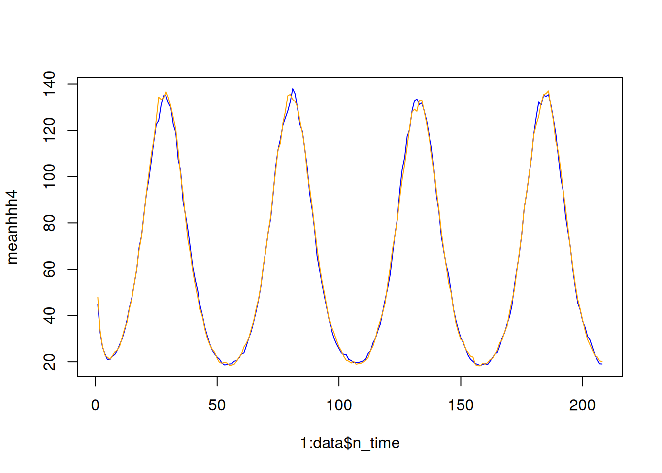
surveillance offers a lot of different plotting functions:
plot(noroEEsim, type = "time")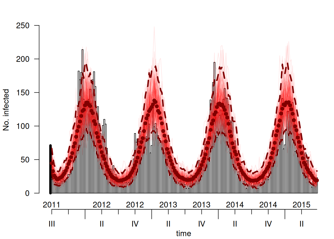
plot(noroEEsim, type = "fan")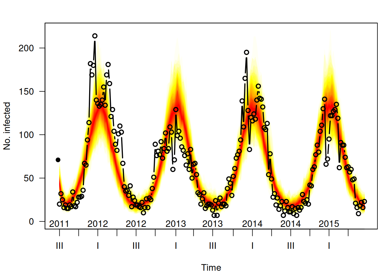
We construct our own plotting function to visualize the simulations aggregated over districts. The function shows the observed number of cases, together with the mean of the simulated values and the corresponding 95% simulation band.
plot.sims <- function(sims, Y, band = 0.95)
{
  obs <- rowSums(Y)
  sim <- apply(sims, c(1, 3), sum)

  m  <- rowMeans(sim)
  lo <- apply(sim, 1, quantile, (1 - band)/2)
  up <- apply(sim, 1, quantile, 1 - (1 - band)/2)

  plot(obs, type = "l", col = 2, lwd = 2,
       ylim = range(c(obs, up)),
       xlab = "Time", ylab="Cases")

  lines(m, col = "darkred", lwd = 2, lty = 3)
  lines(obs, col = "black", lwd = 2)
  lines(lo, col = "darkred", lty = 2, lwd = 2)
  lines(up, col = "darkred", lty = 2, lwd = 2)

  legend("topright",
         legend = c("Observed", "Mean simulation", paste0(band * 100, "% band")),
         col = c("black", "darkred", "darkred"),
         lwd = c(2, 2, 2),
         lty = c(1, 3, 2),
         bty = "n")
}
We then use this function to plot both simulations generated from the RTMB and hhh4 implementations. It’s working seamlessly for both, as the function only relies on the structure of the simulation array.
str(simsEEh) num [1:208, 1:12, 1:100] 1 3 3 1 3 0 0 3 2 2 ...str(noroEEsim, give.attr = FALSE) 'hhh4sims' num [1:208, 1:12, 1:100] 1 3 3 1 3 0 0 3 2 2 ...plot.sims(simsEEh, data$Y)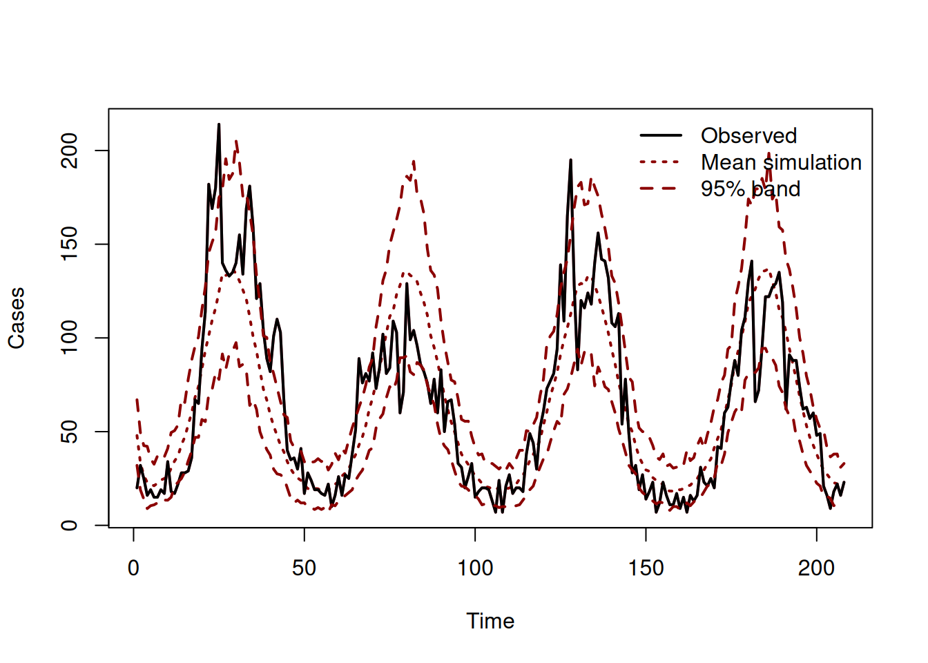
plot.sims(noroEEsim, data$Y)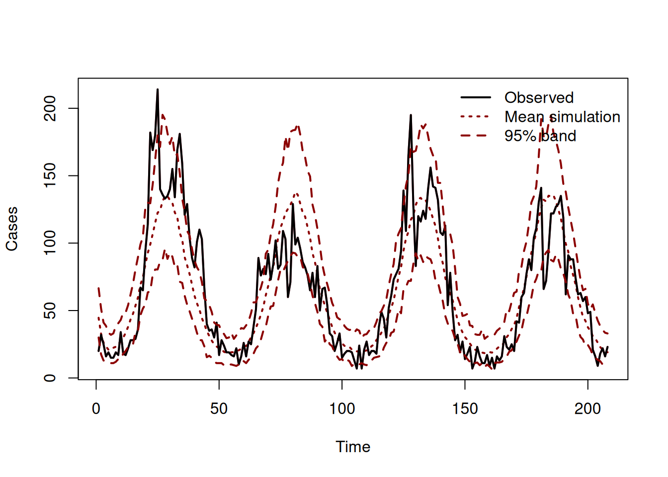
2.6 Would a wrapper for surveillance:::meanHHH() work as a helper function too?
Since just some functions are compatible with the advector class that is used needed the taping for the AD in RTMB or better TMB, to build the AD graph (see: vignette("RTMB-advanced")), the meanHHH() is doing to many operations, that make R to get rid of the advector class.
Here are the methods that work with advectors:
methods(class = "advector") [1] [ [[ [<- %*% aperm
[6] apply as.complex as.double as.vector atan2
[11] besselI besselJ besselK besselY c
[16] cbind chol coerce colSums Complex
[21] cov2cor crossprod dbeta dbinom dcauchy
[26] determinant dexp df dgamma diag
[31] diff dlogis dmultinom dnbinom dnorm
[36] dpois dt dweibull eigen fft
[41] findInterval ifelse is.finite is.infinite is.na
[46] is.nan is.numeric lbeta length<- Math
[51] matrix max mean min Ops
[56] pbeta pbinom pexp pgamma plogis
[61] pnbinom pnorm ppois print prod
[66] pweibull qbeta qexp qgamma qlogis
[71] qnorm qweibull rbind rep rowSums
[76] show solve sort splinefun sum
[81] Summary svd tcrossprod
see '?methods' for accessing help and source codeWe can test meanHHH(), to see where it would break the taping:
end.fe <- rep(0, data$n_unit)
names(end.fe) <- paste0("end.1.", colnames(data$Y))
parms <- c(
  list(ar.1  = 0, ne.1 = 0, end.sin = 0, end.cos = 0),
  as.list(end.fe),
  list(
    neweights.logd = log(2),
    log_overdispersion = 0
  )
)

data1 <- data
data1$hhh4model <- noroEEFit

meanHHHrtmb <- function(parms, data){
  theta <- do.call(c, parms) # theta are the paramters (coefficients)
  model <- terms(data$hhh4model) # are the terms() of the hhh4 model
  surveillance::meanHHH(theta, model, subset=model$subset, total.only=FALSE)
}

objectiveEEhhh4 <- function(parms, data) {
  ## tells RTMB that that Y is the response
  data$Y <- OBS(data$Y)
  print(class(data$Y))
  fit <- meanHHHrtmb(parms, data)
  ## negative log likelihood
  nll <- - sum(dnbinom2(data$Y[-1, ], mu = fit$mean, size = exp(parms$log_overdispersion), log = TRUE))
  return(nll)
}

objEEhhh4 <- MakeADFun(cmb(objectiveEEhhh4, data1), parms)
[1] "matrix" "array" Error in `advector()`:
! Invalid argument to 'advector' (lost class attribute?)This is what traceback() would tell us:
# 14: stop("Invalid argument to 'advector' (lost class attribute?)") at advector.R#13
# 13: advector(e2) at advector.R#78
# 12: Arith2(advector(e1), advector(e2), .Generic) at advector.R#78
# 11: Ops.advector(exppred, offset) at hhh4.R#863
# 10: computePartMean(2) at hhh4.R#868
# 9: surveillance::meanHHH(theta, model, subset = model$subset, total.only = FALSE) at #17
# 8: meanHHHrtmb(parms, data) at #24
# 7: f(p, d) at _setup.R#49
# 6: func(pl) at advector.R#831
# 5: f(x) at advector.R#372
# 4: .MakeTape(mapfunc, obj$env$par) at advector.R#858
# 3: MakeADFunObject(data, parameters, reportenv, ADreport = ADreport,
#        DLL = DLL) at TMB.R#525
# 2: obj$retape() at advector.R#928
# 1: MakeADFun(cmb(objectiveEEhhh4, data), parms) at #30
offset can be of class “advector” and loose it in the neighbourhood part with parameterized power-law weights. We could try a model where we weigh all neighbours the same.
weights <- matrix(1, nrow = data$n_unit, ncol = data$n_unit)
diag(weights) <- 0
noroEEFit2 <-  update(noroEEFit, ne = list(f = ~ 1, weights = weights))
data2 <- data
data2$hhh4model <- noroEEFit2

objEEhhh4 <- MakeADFun(cmb(objectiveEEhhh4, data2), parms[-which(names(parms) == "neweights.logd")])
[1] "matrix" "array" Error in `advector()`:
! Invalid argument to 'advector' (lost class attribute?)This is the traceback() we get now:
# 14: stop("Invalid argument to 'advector' (lost class attribute?)") at advector.R#13
# 13: advector(e2) at advector.R#78
# 12: Arith2(advector(e1), advector(e2), .Generic) at advector.R#78
# 11: Ops.advector(pred, X * fe) at hhh4.R#856
# 10: computePartMean(3) at hhh4.R#869
# 9: surveillance::meanHHH(theta, model, subset = model$subset, total.only = FALSE) at #17
# 8: meanHHHrtmb(parms, data) at #24
# 7: f(p, d) at _setup.R#49
# 6: func(pl) at advector.R#831
# 5: f(x) at advector.R#372
# 4: .MakeTape(mapfunc, obj$env$par) at advector.R#858
# 3: MakeADFunObject(data, parameters, reportenv, ADreport = ADreport,
#        DLL = DLL) at TMB.R#525
# 2: obj$retape() at advector.R#928
# 1: MakeADFun(cmb(objectiveEEhhh4, data2), parms[-which(names(parms) ==
#        "neweights.logd")]) at #7
Somewhere in how we get fe is losing the “advector” class. It could be the subsetting with fe[,which] <- toMatrix(fixed[idxFE==i],c=sum(which)).
A model without fixed effects might work:
noroEEFit3 <-  update(noroEEFit2, end = list(f = addSeason2formula(f = ~ 1)))
data2 <- data
data2$hhh4model <- noroEEFit3
parms3 <- list(
  ar.1  = 0, ne.1 = 0, end.1 = 0,
  end.sin = 0, end.cos = 0,
  log_overdispersion = 0
  )

objEEhhh4 <- MakeADFun(cmb(objectiveEEhhh4, data2), parms3)

## fit the model
ptm <- proc.time()
optEEhhh4 <- nlminb(
  objEEhhh4$par,
  objEEhhh4$fn,
  objEEhhh4$gr
  )
## calculate uncertainties
sdrEEhhh4 <- sdreport(objEEhhh4)
runtime_EEhhh4 <- proc.time() - ptm
run_diffhhh4 <- runtime_EEhhh4 - noroEEFit3$runtime
So this simple endemic-epidemic model runs using RTMB together with surveillance::meanHHH(). It seems to use only AD-compatible functions. Although it’s not really usefull if we can only run such simple models, this is a very nice option for comparing the hhh4 fit and a model with RTMB that use the exactly same math in meanHHH.
Now we can compare the hhh4 model without power law and fixed effects with the RTMB model that uses meanHHH() as a helper function.
| hhh4 | RTMB | diff. | |
|---|---|---|---|
| Parameters | |||
| ar.1 | -0.797933907 (0.046083194) | -0.797933346 (0.046083283) | -5.61e-07 (-8.88e-08) |
| ne.1 | -4.362979051 (0.267831224) | -4.36297355 (0.267840098) | -5.5e-06 (-8.87e-06) |
| end.1 | 0.551595231 (0.092646461) | 0.551590444 (0.092650064) | 4.79e-06 (-3.6e-06) |
| end.sin(2 * pi * t/52) | 0.012659253 (0.053483415) | 0.012660495 (0.053484375) | -1.24e-06 (-9.6e-07) |
| end.cos(2 * pi * t/52) | -0.910723286 (0.045515916) | -0.910721194 (0.045516214) | -2.09e-06 (-2.98e-07) |
| -log(overdisp) | 1.456875107 (0.058041835) | 1.456876005 (0.058041855) | -8.98e-07 (-2e-08) |
| Metrics | |||
| Log-Likelihood | -5874.855973206 | -5874.855973211 | 6e-09 |
| Runtime (seconds) | 0.047 | 0.056 | -0.009 |