library(hhh4addon)
noroEElagModel <-   list(
    end = list(
      f = addSeason2formula(f = ~ -1 + fe(1, unitSpecific = TRUE))),
    ar = list(f = ~ 1),
    ne = list(
      f = ~ 1,
      weights = neighbourhood(noroBE) >= 1),
    family = "NegBin1",
    data = list(t = 1:nrow(noroBE) - 1),
    funct_lag = geometric_lag,
    max_lag = 4,
    subset = 5:nrow(noroBE) # as we have 4 lags we can not model the first 4 time points
)4 Incorporating Higher-Order Lags
We now try to implement an extension to surveillance::hhh4(), called hhh4addon, which extends the functionality to allow higher-order lags.
4.1 Mathematical Formulation
In standard endemic-epidemic models, the epidemic component depends only on the count observed in the previous time period, \(Y_{i,t-1}\). Bracher and Held (2022) introduced higher-order lags to better account for disease-specific serial interval distributions. This is achieved by replacing the single lag with a weighted sum of past counts up to a maximum lag \(K\).
With weighted higher-order lags, the endemic-epidemic model becomes
\[ \mu_{it} = \nu_{it} + \lambda_{it} \sum_{k=1}^{K} u_k Y_{i,t-k} + \phi_{it} \sum_{j \neq i} w_{ji} \sum_{k=1}^{K} u_k Y_{j,t-k}, \]
where the lag weights are constrained to be positive and normalized such that
\[ \sum_{k=1}^{K} u_k = 1. \]
4.1.1 Geometric Lag Structure
Bracher and Held (2022) consider several lag-weight specifications, including parametric ones (e.g., Poisson or linear decay) as well as non-parametric weights. Here, we focus on geometric lag weights.
The geometric weights \(u_d\) depend on a single parameter \(\alpha \in (0,1)\):
\[ u_k = (1-\alpha)^{k-1}\alpha. \]
In hhh4addon, the parameter \(\alpha\) is estimated using a profile likelihood approach. In RTMB, we instead estimate \(\alpha\) jointly with the remaining parameters through the full likelihood.
For a detailed discussion of lag-weight alternatives, see Bracher and Held (2022).
4.2 Using surveillance
The hhh4addon extenstion can be downloaded and installed from github via remotes::install_github("jbracher/hhh4addon"). To fit a higher-order lag model the function profile_par_lag() is used. The control list needs to be extended for the lag function that should be used (funct_lag), the maximum number of lags \(K\) (max_lag) and the which subset is used.
Note
Fitting a lag model in hhh4addon
More information on different arguments and ways to fit a higher-order lag model can be found in the vignette (vignette("hhh4addon")) of hhh4addon.
Since the power-law weights are not helping much with the model, we only weigh each neighbour the same here.
To fit the model the function profile_par_lag() is used. We use the argument return_full_cov = TRUE, to get the standard error of the par_lag parameter estimate (\(\alpha\)).
ptm <- proc.time() # runtime that includes profile likelihood needs to be manually overwritten
noroEElagFit <- profile_par_lag(noroBE, noroEElagModel, return_full_cov = TRUE)
noroEElagFit$best_mod$runtime <- proc.time() - ptm
We need to select best_mod, since the covariance matrix is saved too as cov. The best_mod object is our usual hhh4 fit.
summary(noroEElagFit$best_mod)
Call:
hhh4_lag(stsObj = stsObj, control = control)

Coefficients:
                        Estimate  Std. Error
ar.1                    -0.76703   0.05809
ne.1                    -4.29027   0.22112
end.sin(2 * pi * t/52)   0.12313   0.06607
end.cos(2 * pi * t/52)  -1.08798   0.05246
end.1.chwi               0.28477   0.15900
end.1.frkr              -0.48197   0.26144
end.1.lich               0.32523   0.14882
end.1.mahe               0.11413   0.16503
end.1.mitt               0.26203   0.15609
end.1.neuk               0.14943   0.17160
end.1.pank               1.01880   0.11110
end.1.rein               0.37283   0.15137
end.1.span              -0.14184   0.21459
end.1.zehl               1.08129   0.11395
end.1.scho               0.68024   0.13002
end.1.trko               0.36234   0.15201
overdisp                 0.18030   0.01165

Distributed lags used (max_lag = 4). Weights: 0.58; 0.26; 0.11; 0.05
Use distr_lag() to check the applied lag distribution and parameters.

Log-likelihood:   -5672.32
AIC:              11380.64
BIC:              11485.09

Number of units:        12
Number of time points:  204
We can see, that the spatiotemporal part becomes small (\(exp(ne.1) =\) 0.0137012). This was observed for other higher-order lag models too, which is why a joint epidemic component, where the own region is included in the weights, could be a better choice. Bracher and Held (2022) acutally only used models with a joint epidemic component in their evaluation. We will later in chapter Chapter 6 see how to model one epdidemic component with local and neighbourhood transmission.
Since the parameter \(\alpha\) was not estimated jointly with the other parameters (profile likelihood), it is not found within the coefficients. But we get the different weights and a hint to use distr_lag() to get more information on the parameter.
distr_lag(noroEElagFit$best_mod)$funct_lag
function(par_lag, min_lag, max_lag){
p_lag <- exp(par_lag)/(1 + exp(par_lag))
weights0 <- c(rep(0, min_lag - 1), dgeom((min_lag:max_lag) -
1, p_lag))
weights <- weights0/sum(weights0)
return(weights)
}
<bytecode: 0x5b5a5c7fc6a0>
<environment: namespace:hhh4addon>
$par_lag
[1] 0.2541519
$min_lag
[1] 1
$max_lag
[1] 4We can get the standard error with:
noroEElagFit$best_mod$se_par_lag par_lag
0.208107 When fitting the model without returning the covariance matrix, se_par_lag is NA.
noroEElagFit2 <- profile_par_lag(noroBE, noroEElagModel)
noroEElagFit2$se_par_lag
[1] NA4.3 Using RTMB
In our RTMB implementation we want to use the full likelihood. Since we use RTMB for it’s AD approach, we don’t need to manually write down the first and second derivative of the likelihood function.
We just need to add the parametric geometric lag distribution for the weights to the objective function, add the parameters to the list and add the maximum lag number K to the data list.
We build a helper function for the mean again meanEElag(). The weighted sum of lagged counts, \(\sum_{k=1}^{K} u_k Y_{i,t-k}\), is computed for each time point \(t = K +1, \cdots, T\). In the code this is done by using tlag, which indexes the rows of the output matrix Y_weigh_lag, whereas t = tlag + K gives the corresponding real time point. For each \(t\), data$Y[t - k, ] extracts the observations from the \(K\) preceding time points for all districts. Multiplying the lagged observations by U_n and summing over \(K\) lags makes one lag-weighted count for each district. The resulting vector of length \(I\) is then stored as a row of Y_weigh_lag.
meanEElag <- function(parms, data){
  ## ENDEMIC
  end.fe.vec <- group_par(parms, component = "end", type = "1")
  fe_mat <- matrix(end.fe.vec, nrow = data$n_time, ncol = data$n_unit, byrow = TRUE)
  s_vec <- parms$end.sin * data$Ssin + parms$end.cos * data$Scos
  end.exppred <- exp(fe_mat + s_vec)
  end <- end.exppred[-(1:data$K), ]

  ## EPIDEMIC
  ## transform parameters
  plogis_par_lag <- plogis(parms$par_lag)
  ## higher-order lag weights U for K lags
  k <- 1:data$K
  U <-  (1 - plogis_par_lag)^(k - 1) * plogis_par_lag
  ## weights need to be normalized to sum to 1 (serial interval)
  U_n <- U/ sum(U)
  ADREPORT(U_n)
  ## Compute lag weighted sum of Y
  tplagged <- data$n_time - data$K
  Y_weigh_lag <- matrix(NA, nrow = tplagged, ncol = data$n_unit)
  for (tlag in 1:tplagged) {
    t <- tlag + data$K
    Y_weigh_lag[tlag, ] <- t(U_n) %*% data$Y[t - k, ]
  }
  ## AR
  ar.exppred <- exp(parms$ar.1)
  ar <- ar.exppred * Y_weigh_lag
  ## NE
  ## same weights for all neighbours
  W <- data$W_n >= 1
  ne.exppred <- exp(parms$ne.1)
  ne <- ne.exppred * (Y_weigh_lag %*% W)

  return(list(mu = end + ar + ne,
              end = end,
              epi = ar + ne,
              epi.ar = ar, epi.ne = ne,
              end.exppred = end.exppred,
              ar.exppred = ar.exppred,
              ne.exppred = ne.exppred,
              neW = W))
}
objectiveEElag <- function(parms, data) {
Y <- OBS(data$Y)
## helper function for mean calculation
fit <- meanEElag(parms, data)
## negative log likelihood
nll <- - sum(dnbinom2(Y[-(1:data$K), ], mu = fit$mu, size = exp(parms$log_overdispersion), log = TRUE))
nll
}Additional par_lag parameter (corresponds to \(\alpha\)) in parms.
end.fe.vec <- rep(0, data$n_unit)
names(end.fe.vec) <- paste0("end.1.", colnames(data$Y))

parms <- c(
  list(
    ar.1  = 0,
    ne.1 = 0,
    end.sin = 0,
    end.cos = 0),
  as.list(end.fe.vec),
  list(
  log_overdispersion = 0,
  par_lag = 0.1) # parameter for geometric weights
)
Add the maximum number of lags \(K\) to the data list:
data$K <- 4We again process the objective function using MakeADFun().
objEElag <- MakeADFun(cmb(objectiveEElag, data), parms)We fit the model and calculate uncertainties as before.
ptm <- proc.time() # track runtime
## fit the model
optEElag <- nlminb( objEElag$par, objEElag$fn, objEElag$gr)
## calculate uncertainties
sdrEElag <- sdreport(objEElag)
runtime_EElag <- proc.time() - ptm
We use summary() to get the estimates of the RTMB model. Here, we get the par_lag parameter. Since we use ADREPORT() for the lag weights, we get them too.
summary(sdrEElag) Estimate Std. Error
ar.1 -0.76703907 0.06370460
ne.1 -4.29038026 0.22711892
end.sin 0.12310118 0.06990984
end.cos -1.08797679 0.05407677
end.1.chwi 0.28481728 0.16009125
end.1.frkr -0.48186069 0.26142391
end.1.lich 0.32527984 0.14941554
end.1.mahe 0.11421266 0.16548557
end.1.mitt 0.26210890 0.15682800
end.1.neuk 0.14950240 0.17214735
end.1.pank 1.01883847 0.11320035
end.1.rein 0.37291071 0.15249507
end.1.span -0.14171557 0.21479848
end.1.zehl 1.08132409 0.11727023
end.1.scho 0.68028258 0.13233550
end.1.trko 0.36239197 0.15306979
log_overdispersion 1.71313959 0.06464089
par_lag 0.25415928 0.20810931
U_n 0.58447635 0.04277835
U_n 0.25529928 0.01123732
U_n 0.11151473 0.01797879
U_n 0.04870964 0.01356225We extract the lag weights with ucertainties from the AD object list objEElag and plot them:
lagweights <- data.frame(
  Estimate = sdrEElag$value, # as.list(sdrEElag, "Est", report=TRUE)
  SE = sdrEElag$sd, # as.list(sdrEElag, "Std", report=TRUE)
  Lag = 1:data$K)
ggplot(lagweights, aes(x = Lag, y = Estimate)) +
    geom_line(linewidth = 1, color = "firebrick") +
    geom_point(size = 3, color = "firebrick") +
    geom_errorbar(aes(ymin = Estimate - SE, ymax = Estimate + SE), color = "firebrick", alpha = 0.8) +
    theme_bw()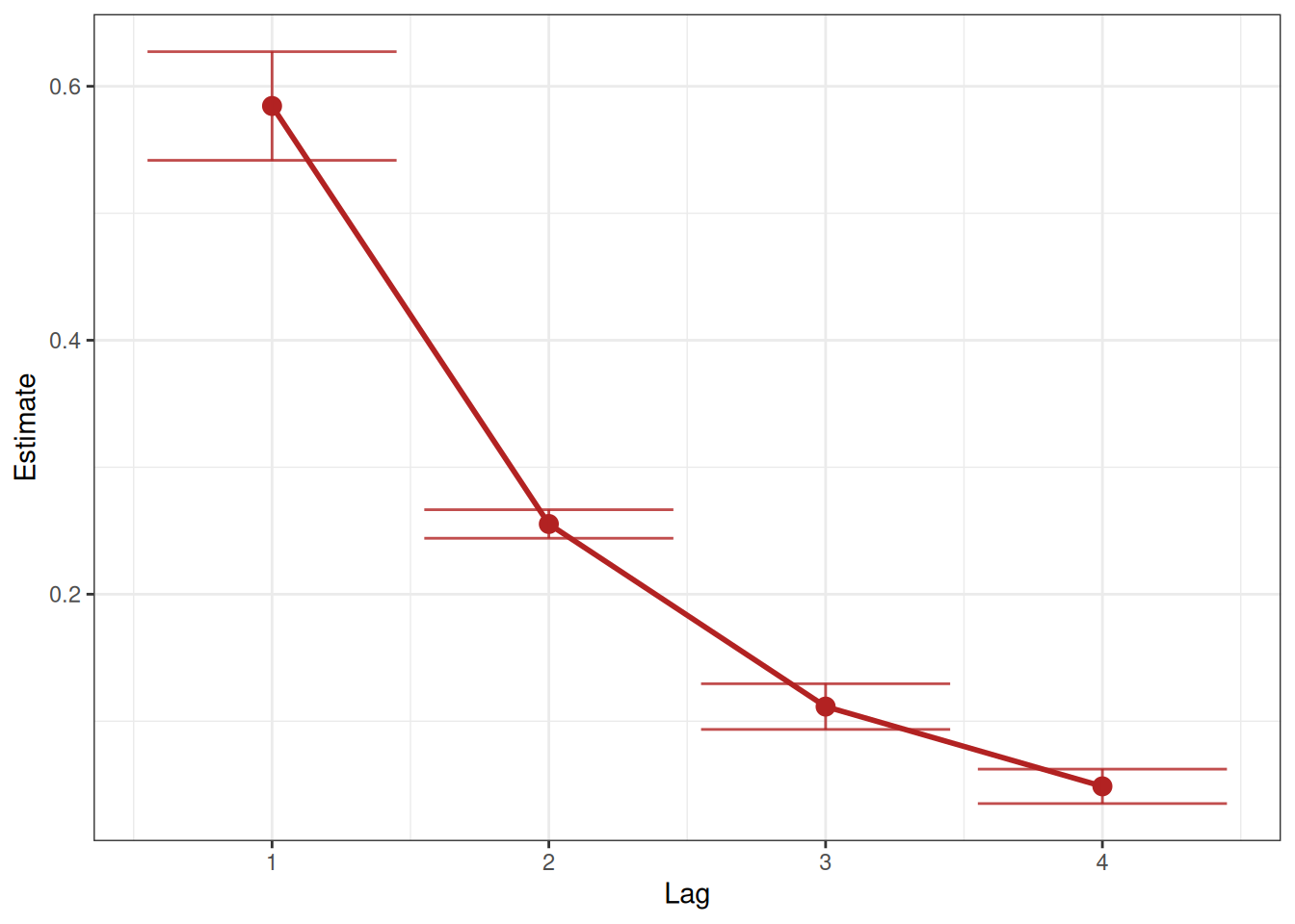
4.4 Comparison Table
| hhh4 | RTMB | diff. | |
|---|---|---|---|
| Parameters | |||
| ar.1 | -0.767032333 (0.058091363) | -0.767039074 (0.063704604) | 6.74e-06 (-0.00561) |
| ne.1 | -4.290269794 (0.221116776) | -4.290380263 (0.227118925) | 0.00011 (-0.006) |
| end.sin(2 * pi * t/52) | 0.12312771 (0.066065948) | 0.123101184 (0.06990984) | 2.65e-05 (-0.00384) |
| end.cos(2 * pi * t/52) | -1.087984654 (0.052455623) | -1.087976795 (0.054076768) | -7.86e-06 (-0.00162) |
| end.1.chwi | 0.284769662 (0.15899581) | 0.284817284 (0.160091249) | -4.76e-05 (-0.0011) |
| end.1.frkr | -0.481972474 (0.261435773) | -0.481860692 (0.261423912) | -0.000112 (1.19e-05) |
| end.1.lich | 0.325225066 (0.148820762) | 0.325279841 (0.149415539) | -5.48e-05 (-0.000595) |
| end.1.mahe | 0.114129888 (0.165031289) | 0.114212662 (0.165485567) | -8.28e-05 (-0.000454) |
| end.1.mitt | 0.26203386 (0.15608937) | 0.262108897 (0.156828005) | -7.5e-05 (-0.000739) |
| end.1.neuk | 0.149432105 (0.171596294) | 0.149502397 (0.172147349) | -7.03e-05 (-0.000551) |
| end.1.pank | 1.018802989 (0.111099651) | 1.01883847 (0.113200354) | -3.55e-05 (-0.0021) |
| end.1.rein | 0.372832259 (0.151369059) | 0.37291071 (0.152495068) | -7.85e-05 (-0.00113) |
| end.1.span | -0.14184098 (0.214589856) | -0.14171557 (0.21479848) | -0.000125 (-0.000209) |
| end.1.zehl | 1.081288106 (0.113949886) | 1.081324092 (0.117270227) | -3.6e-05 (-0.00332) |
| end.1.scho | 0.680242734 (0.130016729) | 0.680282578 (0.1323355) | -3.98e-05 (-0.00232) |
| end.1.trko | 0.362338084 (0.152008407) | 0.362391973 (0.153069793) | -5.39e-05 (-0.00106) |
| -log(overdisp) | 1.713134897 (0.06460219) | 1.713139588 (0.064640894) | -4.69e-06 (-3.87e-05) |
| par_lag | 0.254151861 (0.208106987) | 0.254159281 (0.208109306) | -7.42e-06 (-2.32e-06) |
| Metrics | |||
| Log-Likelihood | -5672.319351629 | -5672.319351882 | 2.53e-07 |
| Runtime (seconds) | 3.994 | 0.163 | 3.831 |
While the estimates and SEs are quite similar, RTMB is faster. This is not suprising, since hhh4addon is estimating par_lag (\(\alpha\)) using profile likelihood, which requires optimizing all other model parameters conditional on different values of \(\alpha\).