3  Incorporating Random Effects

Endemic-epidemic models can also be extended to handle unobserved heterogeneity across regions by introducing random effects into the linear predictors, as established by Paul and Held (2011).

3.1 Mathematical Formulation

Since only the formulation of the linear predictors change, we just look at them. To capture regional variations not explained by covariates, we can add district-specific random intercepts (\(b_i\)) to the log-linear predictors of each component. For simplicity we just show it for the endemic component, which we also use as our example later. \[\log(\nu_{it}) = \beta_0^{(\nu)} + b_i^{(\nu)}\]

Where:

• \(\beta_0\) is the global fixed intercept,

• \(b_i^{(\nu)}\) is the independent and identically distributed (IID) random intercept for district \(i\).

We assume these random intercepts are normally distributed around zero and uncorrelated across components.

More information about random intercepts for hhh4 models (CAR, etc) can be found in Paul and Held (2011) and the hhh4 vignettes.

3.2 Using surveillance

We use the same endemic-epidemic model from before and just add random intercepts to the endemic component, using the ri() function in the formula. This can be done easily with the update() function in surveillance. We don’t need to specify a new control list.

noroEEriFit <- update(
  noroEEFit,
  end = list(f = addSeason2formula(f = ~ - 1 + ri(type = "iid", corr = "none")))
)

summary(noroEEriFit)

Call: 
hhh4(stsObj = object$stsObj, control = control)

Random effects:
            Var    Corr
end.ri(iid) 0.1916     

Fixed effects:
                        Estimate  Std. Error
ar.1                    -1.15194   0.06739  
ne.1                    -1.67581   0.16718  
end.sin(2 * pi * t/52)  -0.07215   0.04031  
end.cos(2 * pi * t/52)  -0.99464   0.03861  
end.ri(iid)              0.64276   0.14679  
neweights.logd          -1.49530   2.33178  
overdisp                 0.19164   0.01214  

Penalized log-likelihood:  -5778.44 
Marginal log-likelihood:   -39.24 

Number of units:        12 
Number of time points:  207 

The global intercept end.ri is shown in the summary as well as the variance. To see the individual deviations for each district of the global intercept, we use the ranef() function.

ranef(noroEEriFit)

end.ri(iid).chwi end.ri(iid).frkr end.ri(iid).lich end.ri(iid).mahe 
     -0.06225989      -0.78545221      -0.06068782      -0.21805723 
end.ri(iid).mitt end.ri(iid).neuk end.ri(iid).pank end.ri(iid).rein 
     -0.11733941      -0.17377112       0.63640874       0.02752094 
end.ri(iid).span end.ri(iid).zehl end.ri(iid).scho end.ri(iid).trko 
     -0.39323483       0.77340037       0.33785807       0.03561439 

In surveillance we can easily plot a map of the random intercepts:

plot(noroEEriFit, type = "ri", component = "end", exp = TRUE)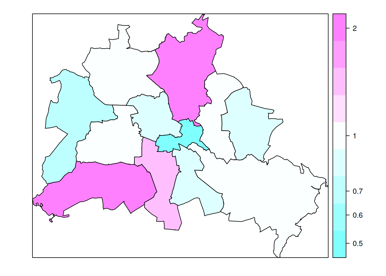

3.3 Using RTMB

If we want to add random effects in RTMB, we just need to add a vector of random intercepts of the length of districts \(i\) in addition to the global intercept, as well as a parameter for the standard deviation of the distribution of the random intercepts.

First, we create a helper function for the mean \(\mu_{it}\):

meanEEri <- function(parms, data){
  ## ENDEMIC
  getAll(parms, data)
  ri_mat <- matrix(end.ri.vec, nrow = n_time, ncol = n_unit, byrow = TRUE)
  s_vec <- end.sin * Ssin + end.cos * Scos
  end.exppred <- exp(end.ri + ri_mat + s_vec)
  end <- end.exppred[-1, ]

  ## EPIDEMIC
  Y_lag <-  Y[1:(n_time - 1), ]
  ar.exppred <- exp(ar.1)
  ar <- ar.exppred * Y_lag

  W <- W_n^(-exp(neweights.logd))
  diag(W) <- 0
  W_norm <- W / rowSums(W)
  ne.exppred <- exp(ne.1)
  ne <- ne.exppred * (Y_lag %*% W_norm)

  return(list(mu = end + ar + ne,
              end = end,
              epi = ar + ne,
              epi.ar = ar, epi.ne = ne,
              end.exppred = end.exppred,
              ar.exppred = ar.exppred,
              ne.exppred = ne.exppred,
              neW = W))
}

We build an objective function using meanEEri(). Here, we need to add the penalization in the log-likelihood, which is the sum of log-density of the random intercepts.

objectiveEEri <- function(parms, data) {

  getAll(parms, data)
  Y <- OBS(Y)
  
  fit <- meanEEri(parms, data)

  ## Initialize negative log likelihood
  nll <- 0

  ## penalization random intercepts
  nll <- nll - sum(dnorm(end.ri.vec, mean = 0, sd = exp(end.ri.sd), log=TRUE))
  REPORT(fit$mu)

  ## negative log likelihood
  nll <- nll - sum(dnbinom2(Y[-1, ], mu = fit$mu, size = exp(log_overdispersion), log = TRUE))
  
  return(nll)
}

We add the random intercept vector and standard deviation to the parameter list:

parms <- list(
  ar.1  = 0, 
  ne.1 = 0, 
  end.sin = 0, 
  end.cos = 0,
  end.ri = 0, # global intercept
  neweights.logd = log(2), 
  log_overdispersion = 0,
  end.ri.vec = diag(data$W_n), # to get a named vector of 0s
  end.ri.sd = 0  
)
## diagonal of neighbourhood matrix is named vector of 0s
diag(data$W_n)

chwi frkr lich mahe mitt neuk pank rein span zehl scho trko 
   0    0    0    0    0    0    0    0    0    0    0    0 

Finally we can process the objective function, where we need to add which our random intercept is, using the random argument:

objEEri <- MakeADFun(cmb(objectiveEEri, data), parms, random = "end.ri.vec")

We fit the model and calculate uncertainties as before.

ptm <- proc.time() # track runtime
## fit the model 
optEEri <- nlminb( objEEri$par, objEEri$fn, objEEri$gr)
## calculate uncertainties
sdrEEri <- sdreport(objEEri)
runtime_EEri <- proc.time() - ptm

We use summary() to get the estimates of the RTMB model. Here we get everything in the order of the given parms list.

summary(sdrEEri)

                      Estimate Std. Error
ar.1               -1.14316597 0.06728866
ne.1               -1.56959201 0.15900895
end.sin            -0.06086412 0.04262330
end.cos            -0.99501939 0.04058070
end.ri              0.58293730 0.15162042
neweights.logd     -1.70215772 2.54499183
log_overdispersion  1.64341142 0.06327162
end.ri.sd          -0.82785463 0.22994131
end.ri.vec         -0.05327835 0.15806521
end.ri.vec         -0.81108640 0.21486455
end.ri.vec         -0.05373716 0.15593932
end.ri.vec         -0.21668062 0.17571221
end.ri.vec         -0.11177964 0.16062392
end.ri.vec         -0.17402361 0.15971358
end.ri.vec          0.66594199 0.15190447
end.ri.vec          0.03744401 0.15562227
end.ri.vec         -0.41090156 0.17463112
end.ri.vec          0.80437956 0.15323840
end.ri.vec          0.36049131 0.15293007
end.ri.vec          0.04467813 0.15691482

If we just print the “sdr” object, we get the parameters without random intercepts similar to the hhh4 summary.

sdrEEri

sdreport(.) result
                      Estimate Std. Error
ar.1               -1.14316597 0.06728866
ne.1               -1.56959201 0.15900895
end.sin            -0.06086412 0.04262330
end.cos            -0.99501939 0.04058070
end.ri              0.58293730 0.15162042
neweights.logd     -1.70215772 2.54499183
log_overdispersion  1.64341142 0.06327162
end.ri.sd          -0.82785463 0.22994131
Maximum gradient component: 0.0002147566 

We can get the random intercepts from the “sdr” object like this:

sdrEEri$par.random

 end.ri.vec  end.ri.vec  end.ri.vec  end.ri.vec  end.ri.vec  end.ri.vec 
-0.05327835 -0.81108640 -0.05373716 -0.21668062 -0.11177964 -0.17402361 
 end.ri.vec  end.ri.vec  end.ri.vec  end.ri.vec  end.ri.vec  end.ri.vec 
 0.66594199  0.03744401 -0.41090156  0.80437956  0.36049131  0.04467813 

Unfortunenately, the names of end.ri.vec specified in parms are lost during the processing.

We could specify the random effects by individual names directly in the parameter list:

end.ri.vec <- rep(0, data$n_unit)
names(end.ri.vec) <- paste0("end.ri.", colnames(data$Y))

parms_i <- c(
  list(
    ar.1  = 0, 
    ne.1 = 0, 
    end.sin = 0, 
    end.cos = 0,
    end.ri = 0, # global intercept
    neweights.logd = log(2),
    log_overdispersion = 0),
  as.list(end.ri.vec),  
  list(end.risd = 0)  
)

Since unlist() is not overloaded for the “advector” class, we use a hacky trick, calling c() with all random intercepts as objects to be concatenated. Otherwise, we would not track the random intercepts specified in parms_i as those in the AD graph (tapeing).

## unlist() is not working for class "advector"
## but "advector" is what is tracked on the tape
group_par <- function(parms, component, type, which = colnames(data$Y), threeparts = TRUE) {
  sepr <- ifelse(threeparts, ".", "")
  parnames <- paste0(component, ".", type, sepr, which)
  return(do.call(c, parms[parnames]))
}

meanEEri_i <- function(parms, data){
  ## ENDEMIC
  end.ri.vec <- group_par(parms, "end", type = "ri")
  print(class(end.ri.vec))
  ri_mat <- matrix(end.ri.vec, nrow = data$n_time - 1, ncol = data$n_unit, byrow = TRUE)
  s_vec <- parms$end.sin * data$Ssin[-1] + parms$end.cos * data$Scos[-1]
  end <- exp(parms$end.ri + ri_mat + s_vec)
  
  ## EPIDEMIC
  Y_lag <-  data$Y[1:(data$n_time - 1), ]
  ar <- exp(parms$ar.1) * Y_lag
  W <- data$W_n^(-exp(parms$neweights.logd))
  diag(W) <- 0
  W_norm <- W / rowSums(W)
  ne <- exp(parms$ne.1) * (Y_lag %*% W_norm)

  return(list(mu = end + ar + ne,
              end = end,
              epi = ar + ne,
              epi.ar = ar,
              epi.ne = ne))
}

objectiveEEri_i <- function(parms, data) {

  data$Y <- OBS(data$Y)

  ## penalization random intercepts
  end.ri.vec <- group_par(parms, "end", type = "ri")
  print(class(end.ri.vec))
  nll <- - sum(dnorm(end.ri.vec, mean = 0, sd = exp(parms$end.risd), log=TRUE))

  ## helper function for mean calculation
  fit <- meanEEri_i(parms, data)
  REPORT(fit$mu)

  ## negative log likelihood
  nll <- nll - sum(dnbinom2(data$Y[-1, ], mu = fit$mu, size = exp(parms$log_overdispersion), log = TRUE))
  
  return(nll)
}

objEEri_i <- MakeADFun(cmb(objectiveEEri_i, data), parms_i, random = "end\\.ri\\.", regexp = TRUE)
ptm <- proc.time() # track runtime
## fit the model 
optEEri_i <- nlminb(objEEri_i$par, objEEri_i$fn, objEEri_i$gr)
## calculate uncertainties
sdrEEri_i <- sdreport(objEEri_i)
runtime_EEri_i <- proc.time() - ptm

summary(sdrEEri_i)

                      Estimate Std. Error
ar.1               -1.14316597 0.06728866
ne.1               -1.56959201 0.15900895
end.sin            -0.06086412 0.04262330
end.cos            -0.99501939 0.04058070
end.ri              0.58293730 0.15162042
neweights.logd     -1.70215772 2.54499183
log_overdispersion  1.64341142 0.06327162
end.risd           -0.82785463 0.22994131
end.ri.chwi        -0.05327835 0.15806521
end.ri.frkr        -0.81108640 0.21486455
end.ri.lich        -0.05373716 0.15593932
end.ri.mahe        -0.21668062 0.17571221
end.ri.mitt        -0.11177964 0.16062392
end.ri.neuk        -0.17402361 0.15971358
end.ri.pank         0.66594199 0.15190447
end.ri.rein         0.03744401 0.15562227
end.ri.span        -0.41090156 0.17463112
end.ri.zehl         0.80437956 0.15323840
end.ri.scho         0.36049131 0.15293007
end.ri.trko         0.04467813 0.15691482

all.equal(unname(sdrEEri_i$par.fixed), unname(sdrEEri$par.fixed))

[1] TRUE

all.equal(unname(sdrEEri_i$par.random), unname(sdrEEri$par.random))

[1] TRUE

Now we have random intercepts named after each district, similar to hhh4. Also we confirm that the results of the two different mean functions are the same.

3.4 Comparing Random Effects

Now, comparing the random intercepts, we see that they are slightly different:

ranef(noroEEriFit) - sdrEEri$par.random

end.ri(iid).chwi end.ri(iid).frkr end.ri(iid).lich end.ri(iid).mahe 
   -0.0089815350     0.0256341861    -0.0069506612    -0.0013766093 
end.ri(iid).mitt end.ri(iid).neuk end.ri(iid).pank end.ri(iid).rein 
   -0.0055597774     0.0002524912    -0.0295332525    -0.0099230732 
end.ri(iid).span end.ri(iid).zehl end.ri(iid).scho end.ri(iid).trko 
    0.0176667314    -0.0309791984    -0.0226332423    -0.0090637418 

3.5 Comparison Table

Parameter estimates and runtime for <code>hhh4</code> and <code>RTMB</code> implementations with standard errors (SE) in brackets and differences between both implementations.

	hhh4	RTMB	diff.
Parameters
ar.1	-1.151944754 (0.067391921)	-1.14316597 (0.067288661)	-0.00878 (0.000103)
ne.1	-1.675806569 (0.167178089)	-1.569592015 (0.159008953)	-0.106 (0.00817)
end.sin(2 * pi * t/52)	-0.072145386 (0.04031047)	-0.06086412 (0.042623297)	-0.0113 (-0.00231)
end.cos(2 * pi * t/52)	-0.994644769 (0.038609056)	-0.995019389 (0.040580695)	0.000375 (-0.00197)
end.ri(iid)	0.642763485 (0.146789015)	0.582937302 (0.151620418)	0.0598 (-0.00483)
neweights.logd	-1.495297213 (2.331782994)	-1.702157718 (2.544991834)	0.207 (-0.213)
-log(overdisp)	1.652151463 (0.063353182)	1.643411422 (0.063271618)	0.00874 (8.16e-05)
end.ri(iid).chwi	-0.062259886 (0.155637505)	-0.053278351 (0.15806521)	-0.00898 (-0.00243)
end.ri(iid).frkr	-0.785452212 (0.199339283)	-0.811086399 (0.214864553)	0.0256 (-0.0155)
end.ri(iid).lich	-0.06068782 (0.153407802)	-0.053737159 (0.15593932)	-0.00695 (-0.00253)
end.ri(iid).mahe	-0.218057227 (0.1719338)	-0.216680618 (0.175712206)	-0.00138 (-0.00378)
end.ri(iid).mitt	-0.117339415 (0.157736552)	-0.111779637 (0.160623917)	-0.00556 (-0.00289)
end.ri(iid).neuk	-0.173771119 (0.156816424)	-0.17402361 (0.15971358)	0.000252 (-0.0029)
end.ri(iid).pank	0.636408739 (0.148154051)	0.665941991 (0.151904468)	-0.0295 (-0.00375)
end.ri(iid).rein	0.027520941 (0.153101183)	0.037444015 (0.155622268)	-0.00992 (-0.00252)
end.ri(iid).span	-0.393234829 (0.168681881)	-0.41090156 (0.174631122)	0.0177 (-0.00595)
end.ri(iid).zehl	0.773400366 (0.14881506)	0.804379565 (0.153238404)	-0.031 (-0.00442)
end.ri(iid).scho	0.33785807 (0.150281072)	0.360491312 (0.152930075)	-0.0226 (-0.00265)
end.ri(iid).trko	0.035614392 (0.154153859)	0.044678133 (0.156914824)	-0.00906 (-0.00276)
Random Effects Variance	0.191570297	0.190956568	0.000613729
Metrics
Log-Likelihood	-5778.442432354	-5797.142934267	18.700501913
Runtime (seconds)	0.457	1.09	-0.633

The difference in the negative log-likelihood is large, with 18.7, although the parameter estimates are quite similar.

We can use the surveillance:::penLogLik() function with the parameters of our RTMB model. We have to use the terms from the noroEEriFit model.

end.ri_sd <- sdrEEri$par.fixed[length(sdrEEri$par.fixed)]
coefs <- summary(sdrEEri)[, "Estimate"]
(coefs <- coefs[-which(names(coefs) == "end.ri.sd")])

              ar.1               ne.1            end.sin            end.cos 
       -1.14316597        -1.56959201        -0.06086412        -0.99501939 
            end.ri     neweights.logd log_overdispersion         end.ri.vec 
        0.58293730        -1.70215772         1.64341142        -0.05327835 
        end.ri.vec         end.ri.vec         end.ri.vec         end.ri.vec 
       -0.81108640        -0.05373716        -0.21668062        -0.11177964 
        end.ri.vec         end.ri.vec         end.ri.vec         end.ri.vec 
       -0.17402361         0.66594199         0.03744401        -0.41090156 
        end.ri.vec         end.ri.vec         end.ri.vec 
        0.80437956         0.36049131         0.04467813 

penLogLikRTMB <- surveillance:::penLogLik(
  theta = coefs,
  sd.corr = end.ri_sd,
  model = terms(noroEEriFit)
)
print(penLogLikRTMB, digits = 12)

[1] -5778.7583852

noroEEriFit$loglikelihood - penLogLikRTMB

[1] 0.3159528

So if we use the same penalized log-likelihood function, we get much closer likelihoods.

Both implemenations use the penalized log-likelihood to obtain parameter estimates in presence of random effects: \[ \ell_{pen}(\beta,b;\Sigma) = \ell(\beta,b) + \log p(b|\Sigma), \] where \(\log(p(b|\Sigma))\) is the penalty term corresponding to the log distribution of the random effect vector \(b.\) Both use Laplace approximation for maximizing (minimizing) the marginal likelihood \[ L_{marg}(\Sigma) = \int exp(\ell_{pen}(\beta,b;\Sigma))d\beta db. \]

But, in hhh4 the “[…] variance components are treated as fixed when estimating the fixed and random effects. The variance components itself are estimated through maximizing the marginal likelihood after integration with respect to the fixed and random effects” (Paul and Held (2011)). So an alternating algorithm is used, further described in the inference part of Paul and Held (2011). Allowing hhh4 to drop terms that are constant in the corresponding iterative step. “First update regression coefficients given the current variance parameters, then update variance components given current regression coefficients via Newton steps. Iterate these two steps until convergence is reached, i.e. parameter estimates no longer change.” (Paul and Held (2011)).

In RTMB, we specify the negative joint log-likelihood as a function of parameters (\(\beta\), in TMB paper \(\theta\)) and random effects (\(b\), in TMB paper \(u\)). The random effects are then integrated out of the marginal likelihood via Laplace approximation: \[ L(\beta) = \int exp(-f(b, \beta))db .\]

The optimization of random effects is performed automatically by the fn (likelihood function) and gr (gradient function). For each evaluation of the marginal likelihood, inner optimization is performed to find the optimal random effects conditional on the current values of the other parameters, including the variance components (Kristensen et al. (2016)).

While the approaches are very similar, the difference is in the procedure. Wherehhh4 uses an alternating algorithm, RTMB performs the optimization of random effect within each evaluation of the marginal likelihood. This can lead to differences in the negative log-likelihood.

Since the parameter estimates are slightly different, we look at the difference in the estimated mean:

est.fixed <- split(sdrEEri$par.fixed, names(sdrEEri$par.fixed))
est.random <- split(sdrEEri$par.random, names(sdrEEri$par.random))

fitted.values <- meanEEri(c(est.fixed, est.random), data)

head(fitted.values$mu - fitted(noroEEriFit))

             chwi         frkr          lich         mahe          mitt
[1,]  0.006068942  0.011236171  0.0067880957  0.009772715  7.634405e-03
[2,]  0.029355445  0.034569513  0.0319267153  0.034427356  2.953338e-02
[3,]  0.018616752  0.023767663  0.0168256677  0.019766583  1.382965e-02
[4,] -0.004102662  0.002337225 -0.0008278179  0.001388850 -3.449048e-05
[5,]  0.005747826  0.011455386  0.0014588205  0.005490621  3.508954e-03
[6,] -0.004870384 -0.001837448 -0.0077968763 -0.003636782 -6.666599e-03
              neuk         pank         rein         span          zehl
[1,]  4.283202e-03  0.001657139  0.004215129  0.003638195 -0.0007812496
[2,]  3.122603e-02  0.028168088  0.027341247  0.026535763  0.0298485970
[3,]  1.389371e-02  0.013032806  0.013686380  0.015835973  0.0105324858
[4,] -3.547448e-03 -0.003080424 -0.004174383 -0.006396883 -0.0019488920
[5,]  5.583251e-05  0.000123934  0.001528364  0.001401550 -0.0024099659
[6,] -8.641756e-03 -0.006584102 -0.008458921 -0.007374049 -0.0116441224
             scho         trko
[1,]  0.005976764  0.005553169
[2,]  0.026080562  0.028741690
[3,]  0.014545971  0.017939961
[4,] -0.002914309 -0.003179647
[5,]  0.002143818  0.003446114
[6,] -0.005273626 -0.005431302

The maximal absolute difference is 0.2210901, which is not negligible.

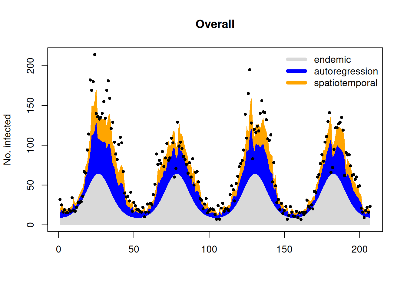
The plots of the total fitted values look the same.

plot(noroEEriFit, type = "fitted", total = TRUE)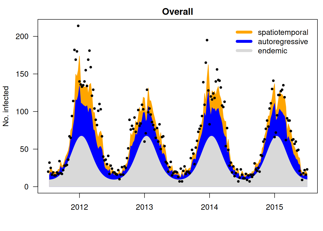

plot.RTMBfit(fitted.values, data)

Kristensen, Kasper, Anders Nielsen, Casper W. Berg, Hans Skaug, and Bradley M. Bell. 2016. “TMB: Automatic Differentiation and Laplace Approximation.” Journal of Statistical Software 70 (April): 1–21. https://doi.org/10.18637/jss.v070.i05.

Paul, M., and L. Held. 2011. “Predictive Assessment of a Non-Linear Random Effects Model for Multivariate Time Series of Infectious Disease Counts.” Statistics in Medicine 30 (10): 1118–36. https://doi.org/10.1002/sim.4177.